How do we represent a rotation in 3 dimensions? This is a surprisingly deep question, and one we can learn a lot from. Our goal will be to “rediscover” quaternions from first principles, building them up by exploring different representations and fixing the failures along the way.
Finding safe representations for 3D rotations has applications in a wide array of areas: 3D modeling software, robot path planning, space navigation, and medicine (e.g., representing the rotation of a scalpel in a robot’s hand), manufacturing, and really any field that works in 3 dimensions.
3D Rotations
Euler Angles
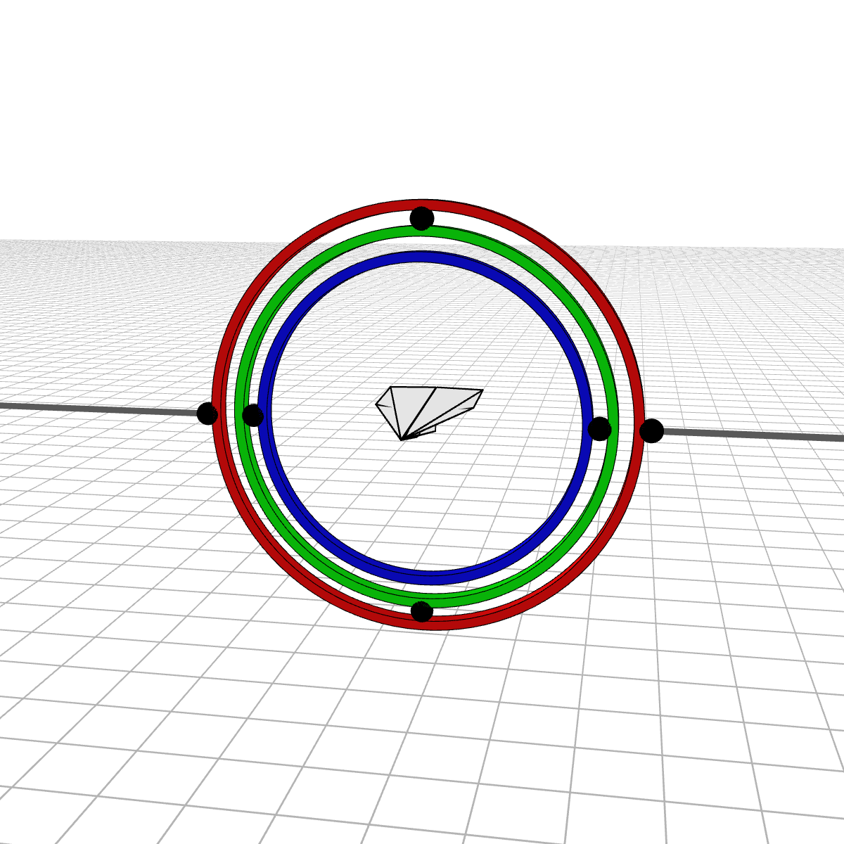
Most people are initially exposed to 3D rotations through Euler angles: Yaw, Pitch, and Roll, so let’s start there. Below we see a gimbal with 3 rings, one for each Euler angle. In the computer we can represent each gimbal (colored ring) with a single value for its angle of rotation. Here is an airplane randomly rotating around, and we also see the associated Euler angles represented with the gimbals.
Every possible 3D rotation can be parameterized using Euler angles, but they have some issues. In certain orientations, the system can get stuck in what is known as gimbal lock, where the mechanism loses a degree of freedom.
When the middle (green) gimbal becomes parallel with the outer-most gimbal (red), then the inner-most gimbal (blue) aligns with the outer-most gimbal, making one of them redundant and the system loses a degree of freedom. You can see below how if you wanted to rotate the airplane along the plane of the screen, you wouldn’t be able to.
Near gimbal lock, some of the rings whip around violently. Here we see the airplane almost pass through such a rotation. In the first example, the airplane is 10 degrees off from passing through gimbal lock, and in the second, it is 1 degree off.
If we tried to rotate the airplane directly through the gimbal lock axis (at 0 degrees), the outermost gimbal would need to flip 180 degrees instantaneously.
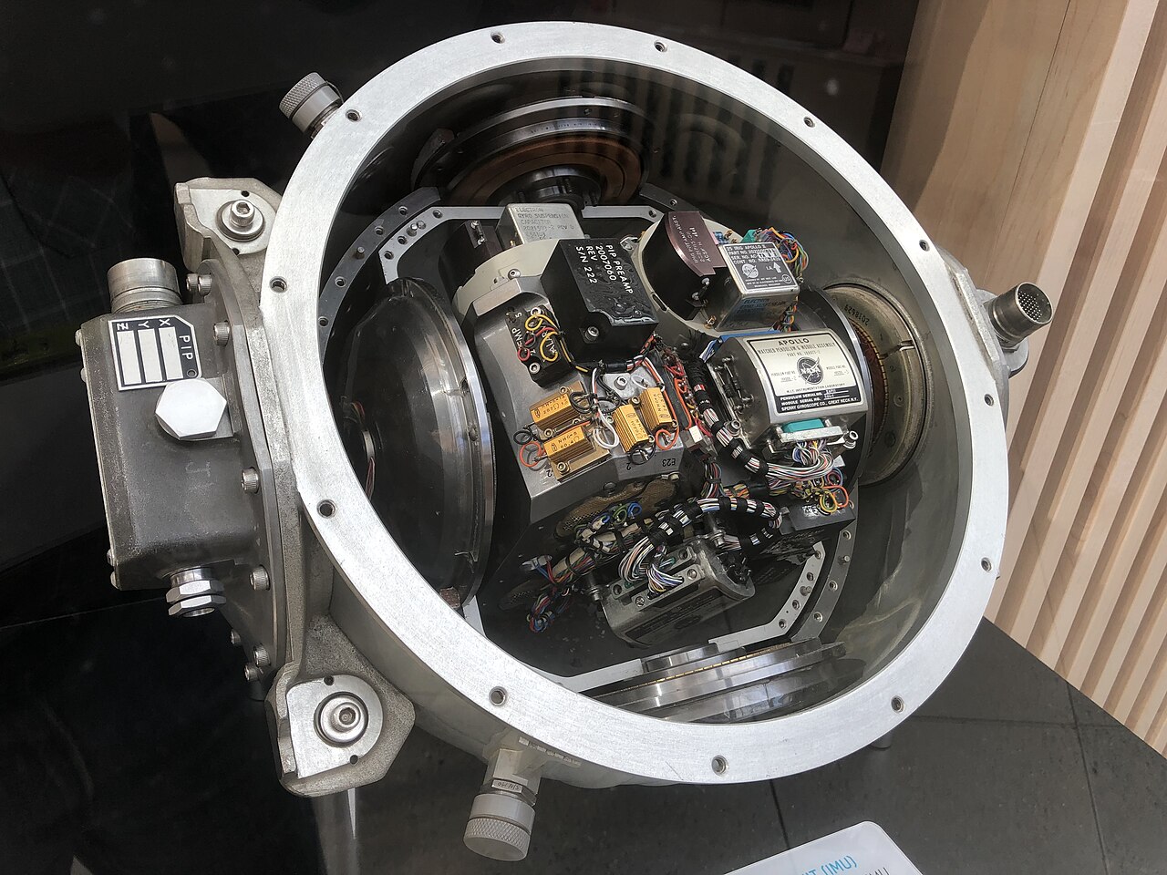
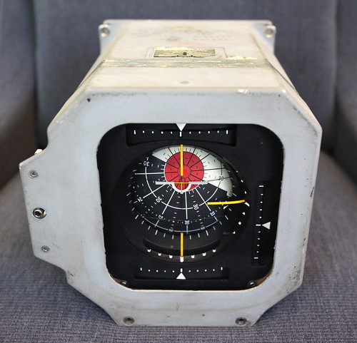
Gimbal lock can cause real issues. On the Apollo 11 mission, astronaut Mike Collins had to manually reorient the spacecraft to prevent its Inertial Measurement Unit (IMU) from entering gimbal lock. He jokingly asked for a fourth gimbal for Christmas, which is one known solution to the issue. You can read the original reasoning as to why they decided to use 3 gimbals instead of 4. Here we see the actual IMU used in Apollo, as well as the Flight Director Attitude Indicator which the astronauts would read to see the Yaw, Pitch, and Roll of the spacecraft. The red spot is the “Gimbal Lock Region”, which if oriented this way, would cause the astronauts to lose attitude navigation, at least until they manually reset it.
These discontinuities are not just an artifact of poor implementation; it can be proven that there will be discontinuities no matter how we implement the Euler angles. We will see later that these singularities will always exist for gimbals, even if we add a fourth gimbal. But to make progress towards quaternions, we will move on to another representation, one which will be the building block on which we can rediscover quaternions.
Rodrigues Vectors
Another possible representation of rotations can be described by an axis to rotate around and an angle for how far to rotate around that axis. This rotation can be represented with a single 3D vector. The direction of the vector indicates the axis to rotate around, and the magnitude describes the angle. This also means that a vector will have a magnitude in $[0, \pi]$. Angles larger then $\pi$ can instead be represented as a smaller rotation around the opposite axis.
Here is the airplane rotating around each of the three axes and the associated Rodrigues vector (also called an axis-angle vector) for that rotation. We also look at random rotations to get a better intuition for what the rotation representation looks like.
We can immediately see discontinuities. While the airplane is rotating continuously, the vector can disappear off one edge of the ball and reappear on the opposite edge. This actually happens at all points on the surface of the ball. Every point on the surface of the ball is equivalent to the point on the opposite point of the ball, which in more formal terms is called “identifying antipodal points”. This identification represents the fact that a rotation by $\pi$ around a given axis is equivalent to a rotation by $\pi$ around the opposite axis.
This gives us a really weird space known as $\mathbb{RP}^{3}$. Imagine this universe where space wraps around at its edges to the other side, where if you walk in any direction long enough you end up back where you started. This almost feels like the sphere which has a similar property, but here in $\mathbb{RP}^{3}$ you would end up back where you started as a mirrored version of yourself. You can see what it looks like to live in $\mathbb{RP}^{3}$ with this shader. This space also describes the unintuitive Dirac Belt Trick, which helps illuminate how strange this space is.
But it still has discontinuities, so what can we do about that? If we look at the same space, but one dimension lower, we can discover a useful trick that we can then apply to this ball.
$\mathbb{RP}^{2}$
A lower-dimensional analog of this space is a circle with opposite edges identified. You could walk off one edge and appear on the opposite edge (and like the ball, mirrored). There are actually many representations of this space you could use, some of which are covered in this delightful old-school educational video.
In our context, this space would represent 3D rotations where one axis is fixed in place. The direction of a vector in this circle represents a 3D axis to rotate around, and the magnitude represents the angle by which to rotate. Here we can see the airplane can rotate along only 2 of its degrees of freedom. We also color the edge of the space such that identified points are the same color.

In this more basic space we can use a clever trick to remove the discontinuities. It’s not possible to embed (read as “stretching”) this space in 3D such that opposite sides of the disk are connected. Although, you can immerse it (read as “stretching with intersections allowed”), which I encourage you to try since it’s a bit mind-bending. What we do to remove the discontinuities is create a second copy of the space and connect the edge on one copy to the opposite edge on the second copy, which can be done by rotating the second copy 180 degrees and connecting the edges together.
This can take a minute to understand, so please stare at the above and below animations for a sufficient amount of time. Below we see a rotation represented in three different ways: a rotated object, the Rodrigues vector, and the two points on the sphere made from the glued-together copies of the Rodrigues vector space. Notice how a rotation is represented twice on this new sphere, which is what allows it to be continuous everywhere.
I also find it helps to think about a few key rotations. The “do nothing” rotation is the center of the circle (zero magnitude vector), which are the poles on the sphere farthest from the rainbow edge represented by the points $(-1, 0, 0)$ and $(1, 0, 0)$. A rotation around the X axis by 90 degrees is represented by the points $(0, 1, 0)$ and $(0, -1, 0)$. The first coordinate is the amount of rotation (representing 0 degrees with 1 and 180 degrees with 0) and the remaining coordinates (normalized) represent the axis we are rotating around.
A nice way to map a point on the disk to a point on the sphere is by $(\text{cos}(\frac{\theta}{2}), \text{sin}(\frac{\theta}{2}) \bf u)$ where $\theta$ is the magnitude of the vector on the disk and $\bf u$ is the normalized vector. Notice that the first coordinate is representing the angle of rotation like we wanted, as in, mapping a do-nothing rotation to $1$ and an 180 degree rotation to $0$.
And now that we have this trick, we can go back to the ball we had earlier with identified antipodal points.
Quaternions
We can take the mapping we used to turn $\mathbb{RP}^{2}$ into the sphere and apply the same mapping from the full 3D rotation space, the 3D ball with identified antipodal points known as $\mathbb{RP}^{3}$, into a 4D sphere. You take two copies of the ball, rotate one by 180 degrees, then connect them in the fourth dimension as a 4D sphere. This creates a 4D sphere, where each rotation is represented exactly twice as antipodal points. We can’t visualize this, but keep in mind that it acts exactly the same as the lower-dimension version we just saw.
This point on the 4D sphere is the quaternion that most people use to represent 3D rotations. When you see a quaternion from now on, you can recall
- The first coordinate $\bf q_w$ is the amount of rotation being applied around an axis. $\theta = 2 \cdot \text{acos}({\bf q_w})$, so the value 1 represents no rotation, and 0 represents a 180 degree rotation.
- The last three coordinates normalized represent the axis to rotate around in 3 dimensions.
- Each 3D rotation has two quaternions to represent it, $\bf q$ and $\bf -q$.
I should mention that there are other representations of 3D rotations, including 3x3 matrices and bi-vectors, but we focused on quaternions since they are one of the most common representations.
All the code used to generate the animations can be found here.
While this completes the main point of the post, I think it would be fun to look at how we could fix the gimbal-lock on Apollo 11.
Fixing the gimbal
Recall that astronaut Mike Collins asked for a fourth gimbal in order to avoid gimbal lock and discontinuities, how does a fourth gimbal fix the issue?
For three gimbals we had a unique set of angles that represented a rotation, so by adding a fourth gimbal we enable a rotation to be represented by many different possible sets of angles. Below we see how the airplane is staying still while the gimbals can move (not at any angle, they still need to produce the desired rotation, but we still see how there is more then one set of angles to map to a rotation).
With this additional degree of freedom, we can now steer around singularities. Imagine we get too close to a singularity, then we just pause the object rotating and move the gimbals around until we’re farther from the singularity, then continue the rotation. But ideally, we don’t have to pause the rotation. There might be a way to map quaternions to 4-DOF gimbals that eliminates the singularities altogether. So, what does such a mapping look like?
It turns out, no such mapping exist, not even if we add more gimbals. You can dive into the details if you like (theorem 1.3 in these notes), but essentially it is because it’s not possible to map a set of $N$ gimbals (represented by the space $T^{2N}$ since we take the product of $N$ unit circles) to the space of rotations ($\mathbb{RP}^{3}$) without introducing singularities.
But not all is lost. We can construct a function that maps the desired rotation with the current gimbal angles into the next gimbal angles. Essentially, this is a function that depends on where the gimbal currently is in order to determine where it should be next. This has the funny implication that we can rotate an object around and return it to its original orientation, but the gimbals may not be in the same orientation.
Below we see the airplane moving randomly as we adjust the gimbals to avoid singularities. Every frame we calculate the set of angles that maximizes the distance to a singularity (the determinant of the Jacobian matrix) while always satisfying our desired rotation.
Long ago NASA had theoretical results on 4-DOF gimbals (also called 4-axis gimbals), and since then there has been an abundance of results on singularity avoidance in gimbal systems of all kinds.
This type of problem is often found in the field of robotics, so if you want to explore more on the movement of robots, I found this textbook very well-written and useful.