Collision Avoidance

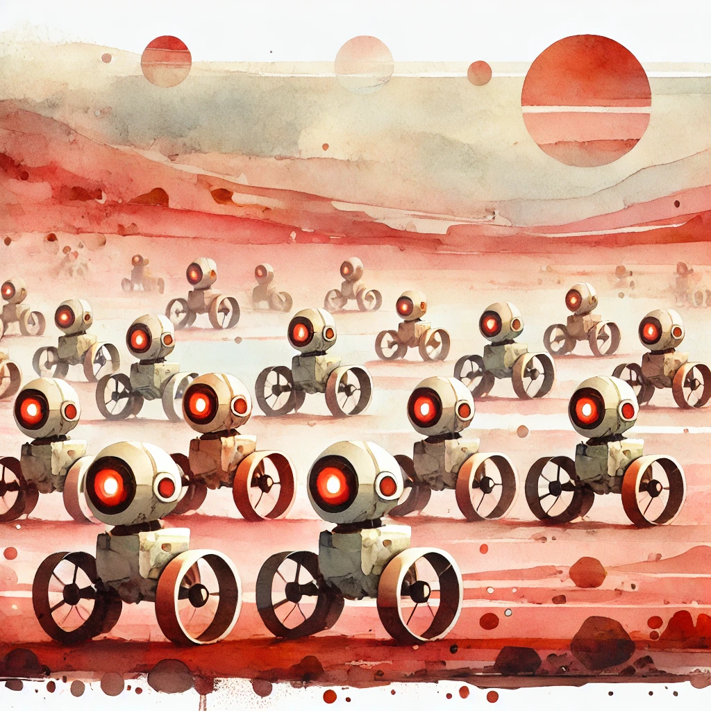
When you’re walking through a large crowd, how do you avoid colliding with everyone else? You aren’t communicating with each other, and you aren’t being directed by a central director, so how does the large crowd coordinate? Everyone is reacting independently using only their visual senses to estimate the velocity and size of everyone else, using that information to plan out a path to some goal.

Let’s find an algorithm so we can let robots navigate crowds as well!

This is a toy model and investigation, and as such we make some pretty simplifying assumptions. We assume everyone is a circle and that robots can perfectly sense other robots velocity and size. To make it a bit more interesting we add noise to all velocities (this has the added benefit of removing unstable equilibriums that can occur in simulations like this), and we don’t let robots change their velocity instantaneously (more details later).

Avoid Nearest Neighbor

The most basic algorithm we can implement is ‘Avoid Nearest Neighbor’. Here’s how we could implement it: Travel towards our goal, but if we get too close to another robot, push away.

We calculate two vectors: The goal vector which points at the goal at max speed, and the evasion vector which points away from the nearest robot. The magnitude of the evasion vector is determined by our distance to the other robot. We want to ensure we never collide, so the magnitude should approach infinity as we approach a collision. A good equation to satisfy these requirements is below, where $p_i$ is the position of the $i$th robot, and $r_i$ is its radius.

\[\text{evasion vector magnitude} = \frac{1}{\left\lVert p_{\text{self}} - p_{\text{closest}} \right\rVert - ( r_{\text{self}} + r_{\text{closest}})}\]

Which means when the two robots are far apart, the magnitude is nearly zero, and when they approach touching, the magnitude approaches infinity.

Now we just add the two vectors together, limit the new vectors magnitude to the robots max velocity, and we have a collision avoidant robot. The scale of each vector can be controlled by a coefficient, and the ratio between these coefficient we will call the evasion strength. When evasion strength is high, it means the evasion vector is weighted much more strongly then the goal vector.

Here is a robot trying to reach a goal with an obstacle in the way. The first is at a low evasion strength and the second is at a high evasion strength.

Note that a higher evasion strength means we are safer, but take longer to reach our goal.

To test this algorithm in crowd-like settings, let’s put 50 robots in a circle and have each one try to get to the opposite side.

It’s not bad, but we see an issue where some robots get nearly to their goal, but get repelled by other robots sitting too close by. We can fix this be using a dynamic evasion strength value. As we get closer to our goal we decrease the evasion strength, until near our goal we arne’t evading at all.

That looks pretty good! But we can still do better.

Velocity Obstacle

We can calculate the valid velocities that ensure a collision won’t occur between any robots, even while they’re moving. This is known as a Velocity Object (VO). VO has been used in maritime calculations since at least 1903 with a neat looking Battenberg’s Course Indicator on a Maneuvering Board. Here’s how it works.

The most simple case is where we consider a point and its valid velocities that avoid colliding it with a static circle. That’s not too hard, it’s just the cone originating at the point and enveloping the circle. Clearly if we set our velocity anywhere in the cone, we will collide with the circle (the red arrow below), and anywhere outside the cone will avoid a collision (green velocity).

If instead of a point we consider the valid velocities of a circle, we need to add an extra step. First notice that for any two circles that are just touching, if we shrink the radius of one and increase the radius of the other in equal parts, the circles will still be touching. This means for the sake of the cone calculation we can shrink our robot down to a point as long as we increase the radius of other robots by the same amount, and we reduced the problem to a point and circle (for more general shapes, look into the Minkowski Sum).

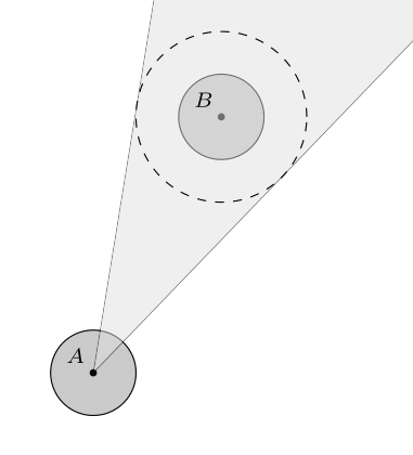
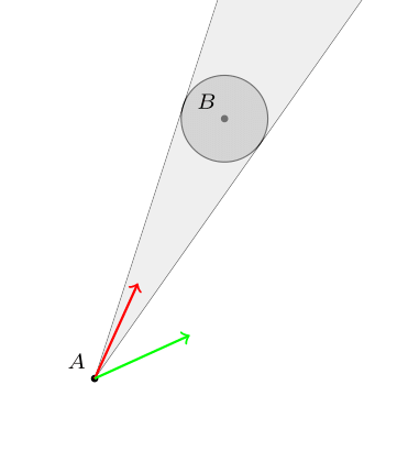
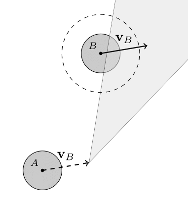
And finally, what if the other circle is moving at a constant velocity? Notice if we were also traveling at the same velocity, from our new frame of reference it looks as if the other robot is standing still. We can calculate the cone again, but then we need to shift the frame of reference back, meaning we also shift the collision cone. This shift will be equal to the velocity of the other robot ($v_B$ in the figure below).

That is the core of VO and all of its variants. We can now apply VO to all the robots around us and find which velocities are valid or invalid.

But that still leaves us the decision for which velocity to actually pick. One solution is to pick the velocity closest to the preferred velocity (the one pointing directly at the goal at max speed) that’s not restricted by any VOs. This has the downside that sometimes there are so many robots around us that no velocities are valid. So instead, we will sample many different potential velocities and score each sample velocity based on how well it points at the goal and how well it avoids collisions.

Sampling Velocities

First we need a way to generate all the sample velocities. We want a sampling of velocities within our max speed and preferably uniformly distributed. The first and easiest way to generate the points would be use two for loops that iterate over angles and radiuses. But here’s a better solution, using the most irrational number (the golden ratio) to uniformly generate points on a disk. You can see how much better it is compared to the naive sampling below, both using the same number of sample points.

for (let radius = 0; radius < 1; radius += 1/10) {
  for (let angle = 0; angle < 2*PI; angle += 2*PI/100) {
    point(radius*cos(angle), radius*sin(angle));
  }
}

for (let index = 0; index < 1000; index++) {
  let radius = sqrt(index / 1000);
  let angle = index * 2*PI * PHI;
  point(radius*cos(angle), radius*sin(angle));
}

And now we need to score each of these potential velocities. We pick the velocity with the least penalty, where the penalty is below. The $v_{\text{preferred}}$ is the vector pointing towards the goal at max speed, $v_{\text{sample}}$ is the velocity we are sampling, and $t_{\text{collision}}$ is the time to the nearest collision for this sample velocity (scored as $\infty$ for no collision).

\[v_{\text{sample}} \ \text{ penalty} = \left\lVert v_{\text{preferred}} - v_{\text{sample}} \right\rVert + \frac{\text{evasion strength}}{t_{\text{collision}}}\]

This has many desirable properties: the penalty approaches infinity as a robot approaches a collision, it scores the preferred velocity with the lowest penalty in the absence of obstacles, and we can use our previous evasion score in a similar way to control how aggressive each robot is.

And with all that, we can run some simulations and see what happens!

Simulations

Again let’s see what effect the evasion strength has on a robot getting around an obstacle. First is the low evasion strength followed by a higher value. Let’s also look at what the sampled velocities scores look like.

And how about two robots trying to pass each other? We should expect the VOs to be offset by the other robots velocity.

And lets go to the crowded circle again! The sampled points will clutter the screen, so let’s remove those.

This looks much nicer then the previous collision avoidance algorithm. But I should now explain the velocity smoothing I mentioned earlier, it plays an important role here. VO has a well-known oscillation issue that arises from two robots constantly flip-flopping their velocities that I tried to avoid with the smoothing. Here’s how the issue arises: Look to the two robots heading directly towards one-another in the figure below, they must choose a velocity outside of the VO (the next velocity we label with a prime), which means both are no longer pointed at one-another, meaning they can each go back to their preferred velocity, only to repeat the process.

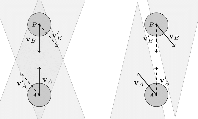
This figure is inspired from the paper that solved this issue, where a modification of VO was proposed called Reciprocal Velocity Obstacles (RVO), and who’s details can be found here. But we took a different approach (mostly just because I thought it would be fun).

We smooth the robots velocity so it can’t make discontinuous jumps, which avoids the oscillations if we smooth it over enough frames (the simulation is inherently discrete, so smoothing can only occur across multiple frames). The robot has a target velocity and a real velocity, where the target velocity can make discontinuous jumps, bu the real velocity must smoothly follow the target velocity. This means oscillations can no longer occur since at some point along the way from our current velocity to the target velocity we will hit a stable velocity, and the oscillation disappears.

To see how the smoothing is implemented and some potential alternatives.

We can firstly simplify the problem into a one-dimension problem since we can smooth the components of our velocity vector independently.

A common smoothing algorithm for a live data-stream is a Simple Moving Average, which takes the average of the last $k$ data points. This is pretty nice, but it’s not as smooth as we might like and requires storing $k$ data points. Below we see the governing equation, where $x_i$ is the $i$th input signal.

$y_t = \frac{1}{k} \sum_{i=0}^{k-1} x_{t-i}$

We could instead take a Weighted Moving Average of the last $k$ points, where we assign small weights to the most recent and oldest points, and weight most heavily the middle of the $k$ points. This would give us a much smoother signal, and we can even control how quickly it smooths. This is an example of a convolution, which is a very powerful tool capable of much more then just smoothing. Below we sample the weights from a gaussian centered at $k/2$.

$y_t = \sum_{i=0}^{k-1} w_i \cdot x_{t-i}$

But these methods require storing $k$ points, it would be nice to do it with even fewer (just for the sake of elegance).

If we use Exponential Smoothing then we only have to store the previous result. For an $\alpha$ value we can control how quickly it reacts to a change in signal. This does have an issue where it isn’t very smooth near the discontinuous change in the input signal, but it is one step closer.

$y_t = (\alpha - 1) y_{t-1} + \alpha x_t$

My favorite implementation is the critically damped oscillator. It requires storing two values, the previous result and its velocity. We imagine the input signal is the source of a spring and our current value is a block attached to the other end of the spring. By dampening the spring we can remove oscillations, and by critically dampening the spring we can reach the target signal as quickly as possible. The spring constant is a parameter we have control over to choose how quickly we react to changes in the signal.

\[y_t = y_{t-1} + v_{t-1} \Delta t\]

$v_t = v_{t-1} + \left( k (x_t - y_{t-1}) - v_{t-1} 2\sqrt{k} \right) \Delta t$

This is in my personal opinion the nicest looking curve for smoothing the velocities, but there really is no best answer here since this a matter of aesthetics.

The code to generate these signals is included at the link at the end.

And now we can run lots of experiments and see what happens.

And we can compare to the initial algorithm that just avoided the nearest neighbor.

These experiments did reveal to me that there is no set of parameters that works perfectly well for all simulations. Some of them were smoother if the evasion strength was larger or smaller, or the smoothing of the velocity was too high (collisions occur) or too low (re-introduced oscillations), or the evasion strength was too high (robots were too close to each other and no one could reach their goal) or too low (robots got too close and collided due to the noise added to the velocity).

All code for these simulations and figures can be found at this repo on my Github.

Limits

This is a collision avoidance algorithm only for local collisions, it needs to be directed by a higher-order system like a path-finding algorithm to determine what the desired velocity is. VO on its own just points at the goal, which would fail for example in a maze.

VO doesn’t handle deadlocks with other robots. You can imagine two robots meeting in a hallway which is too small for either to pass. This is being worked on right now with papers like Adaptive Optimal Collision Avoidance driven by Opinion (AVOCADO).

Future Ideas

Working more on an adaptive evasion strength could allow for robot swarms to collectively complete a task faster. If for example the evasion strength is inversely proportional to your distance to your goal (the opposite of what we have been doing, but this is at a larger scale), then robots who need to get to a farther goal will be given right of way. This hopefully would have the overall effect of speeding up the entire robot swarm.

Similarly, you may want an adaptive evasion strength that depends on how long you’ve been deadlocked for. A small evasion strength is less safe, but may be necessary in cases like getting through tight spaces. A good heuristic may be that the longer you are stuck for, the more aggressive you should try to be.

An interesting problem would be to avoid collisions while also maintaining a cluster of robots. There could be a restraint where a group of robots needs to stay together while avoiding collisions on the way to their destination (like a family in a crowd).

A much more complicated alternative to VO would be to generate a 3D spacetime representation of the available space, and path-find (restricting the path to travel at the robots max speed along the time dimension). This would solve the collisions, high-level path-finding, and deadlocks. Although it may introduce oscillation issues like seen in the original VO. This idea is not new, but generalizing to more environments is still being solved right now.

Collision Avoidance

Avoid Nearest Neighbor

Velocity Obstacle

Sampling Velocities

Simulations

Limits

Future Ideas

Further Reading

Further Reading

Dynamic Decentralized Cluster Identification

A Control Principle Used by Ants and the Internet

Simple Bee-Inspired Swarming