
Problem Statement
We have a bunch of small identical radios with LEDs, and we want to animate them as if they were one giant screen. This means we need to know the physical location of each radio relative to one-another. But these radios don’t have GPS, so all we get to know is the logical topology of the network.
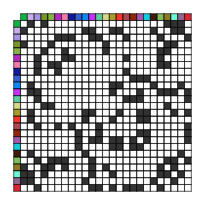
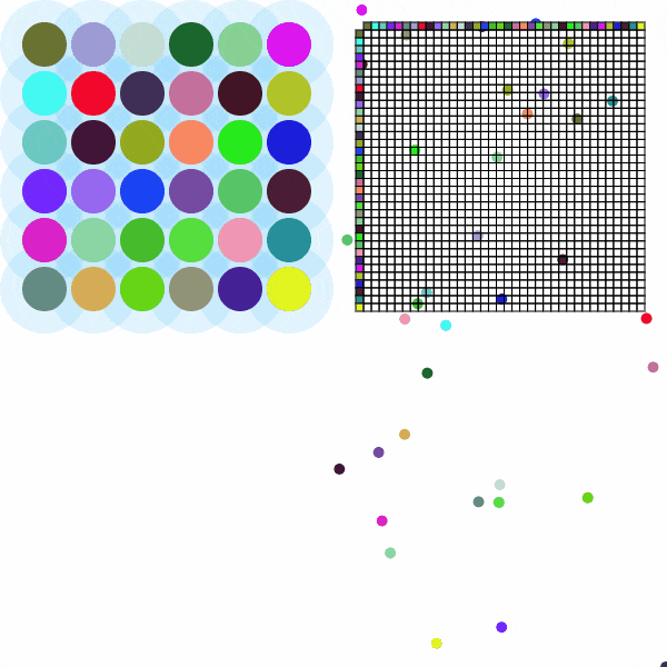
For example, if given the following adjacency matrix (The X and Y axis show each radio as a unique color, and a black grid square means those two radios are within communication range of one-another), what might the physical topology be?
Answer:
It’s not at all obvious, but this is a square grid of radios.
If you sort the columns rather then display them in random order, you can start to tell this is fairly symmetric topology.
You might notice that for some configurations, this problem is impossible to solve. When all the nodes are very close (so the adjacency matrix is completely filled in), or all very far from each other (the adjacency matrix is nowhere filled in), it’s impossible for us to say where the nodes might be relative to each other, as we just don’t have enough information.
In spite of this, might we find a satisfactory way to get a best-effort solution?
Force Directed Graphs
How about we run a physical simulation and see if the computer can just stumble upon a good solution?
Initially, lets place all the nodes on the screen at random, and then we apply forces and let the simulation play out. Here are the rules we will use:
- If a node is connected to another node, apply a force that pulls those nodes towards each other. For aesthetic reasons we actually pull the nodes within a set radius of one-another, so as to not have them get too close.
- If two nodes are not connected, apply a force pushing them apart. The push is stronger the closer they are, and very weak when far apart.
- Add a dampening force so we minimize oscillations.
We should expect to see the nodes move into fairly valid solutions. Here’s an interactive demo where you can move the physical nodes (large nodes) around on screen, and see the adjacency matrix update, and consequently, the force directed graph as well (small nodes).
One interesting question to ask is for what configurations does the force directed graph give reasonable solutions? We already know in extreme cases (fully connected or no connections) the force directed graph will be useless, so at what point do we enter a reasonable range? As just one example to investigate, we look at the grid. We slowly increase the communication range, spanning from no connections to fully connected. Note that we don’t restart the simulation every time, so at every step the graph is transitioning from an already reasonable state, not just random placement.
We see for this size grid, for these force directed graph parameters, with slow transitions between each communication range increase, that the solution seems reasonable when the degree of the central node is within range of 4-12, and fails for 0 (which we expected) and above 12 (which notably is not fully connected, as we can see in the adjacency matrix). It would be interesting to see more tests with varied parameters (random seeds, force graph parameters, topologies, etc.), and with a more reasonable metric then “looks about right”.
You may have noticed another issue with these force directed graphs, which is that they sometimes get twisted. If two chunks of the graph form correctly, but one clockwise and the other counter-clockwise, then one of the chunks is going to have to flip itself, which it won’t do since the force directed graph gets stuck in local minimums. One solution for this is to form the graph one node at a time. Start with placing a random node, then placing one of its connected nodes nearby. If you wait until the graph settles down (minimal movement after a threshold of time), then add the next node, and this process can be repeated until all nodes have been added. This will avoid the clockwise-counter-clockwise problem since the whole topology was built slowly from a small genesis of nodes, which was either clockwise or counter-clockwise, and the clockwise-ness (known as chirality) is maintained throughout the slow build.
Numerical Solution
It would be helpful if we could explicitly state all possible solutions. It will be easier to start with the simplistic case of one dimension, where each node has its position described by just one number. We assume the communication range is $1$ since the units are arbitrary.
We start with just two nodes $(N_a, N_b)$ with positions $(x_a, x_b)$.
- If $N_b$ is connected to $N_a$, then we know $x_b$ is in the range $(x_a-1,x_a+1)$.
- If $N_b$ is not connected to $N_a$, then we know $x_b$ is in the range $(-\infty,x_a-1)$ or $(x_a+1, \infty)$.
Finding the governing inequalities can be easily generalized to a greater number of nodes and higher dimensions. For each pair of nodes $(N_i, N_j)$, if the nodes are connected, then $d(N_a, N_b) < 1$, if they are not connected, then $d(N_a, N_b) > 1$, where $d$ is the distance function.
Expanding this out for the two-node one-dimensional case with positions $(x_a, x_b)$ gives us: When nodes are connected, $x_a < x_b + 1$ and $x_a > x_b - 1$, and when not connected, $x_a > x_b + 1$ or $x_a < x_b - 1$. This is equivalent to the ranges we saw above.
Expanding this out for the two-node one-dimensional case with positions $((x_a, y_a), (x_b, y_b))$ gives us: When nodes are connected, $\sqrt{(x_a-x_b)^2 + (y_a-y_b)^2} < 1$, and when not connected, $\sqrt{(x_a-x_b)^2 + (y_a-y_b)^2} > 1$.
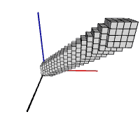
Let’s consider the three-node one-dimensional case and visualize the inequalities. There are 8 possible cases (3 edges, each either connected or not), but many of these are equivalent up to node renaming, so we only need to consider four cases (zero, one, two, and three connections). Here are the solution spaces for each case (approximated with boxes, where a box indicates the inequality is satisfied).
This description of the problem isn’t all that enlightening, but it does formalize the problem, which opens the door for finding more mathematical tools which can make more progress then our intuition might.