Simulated Economy (1)

Concept

Motivation

Imagine an open world RPG where your actions affect the price of goods, the markets reacting to anything the player may do (burn down wheat fields, cost of food increases; kill the merchants, prices differentiate between cities; sell the many swords you’ve collected on your adventures, tank the sword market). What would it take to have such an adaptive simulated economy? You could take a very simple approach and define a rule like The cost of a good is inversely proportional to the amount of that good in the game. But this will inevitable fail to capture the complex behavior we know economies to have. In order to create the desired emergent behavior, we must think at the level of the individual. By the end of this project we’ll have markets that converge to optimal prices, multiple coupled markets, inflation, geographically distinct economies, and merchants connecting cities, all of which adapts to any possible change in the environment. This work is in part inspired by Simulating Supply and Demand and Emergent Economies for Role Playing Games, both great resources if you want to explore more.

We want a complex economy to emerge from simple actions taken by individuals, so how do people make economic decisions? This is an unimaginably deep question, so we need to start somewhere simple. Below is the motivating example to start off our economic model, but keep in mind there are many other approaches.

You’re checking out a new super market in the neighborhood and see your favorite cereal, but then you see that it costs \$10. “This is madness!” you think. You know that just down the road your usual super market sells the same cereal for \$5, so you don’t buy the cereal. But the next day, at your usual super market, you find the price of cereal is now \$10 as well. “This is unfortunate, but it seems the price of cereal has gone up, darn.” You still decide to buy the cereal since you really like it.

This story outlines a very simple decision making algorithm, which although incomplete, gives us a great place to start. People seem to track two numbers when it comes to the price of a good: How much they personally value a good, and how much they expect that good to cost in the market. In the above story, our individual personally valued the cereal at more then \$10, which we know since they eventually bought the cereal for \$10. But this value alone is not enough to explain our story, if it were, then our individual would have immediately bought the cereal from the first market. Their expected market value of the cereal was much lower then the price they saw, so they knew they could probably buy it somewhere else for much cheaper, and that’s why they didn’t buy the first cereal. These two numbers are where we begin.

Implementation

We will begin with a single market. Each actor will keep track of how much they personally value a good and how much they expect that good to cost. From here we can tell if they are a buyer or seller: A buyer is someone who personally values a good more then they expect it to cost (for example, if they value a good at \$10 and expect it to cost \$8 in the market, then they are a buyer of that good), and a seller is someone who values a good less then what they expect it to cost in the market.

This very first simulation will be as simple as possible, no money is given in a trade, no limited goods, no transaction costs, no diminishing returns, nothing except transaction offers. They will attempt to buy and sell with each other at random. But how does the expected market value change over time? In order to have a convergence of prices, we will have the buyer decrease their expected price after a transaction, and sellers increase their price. Essentially, the buyer is thinking “I bought this good for \$10, next time I’ll try and buy it for \$9”, while the seller thinks “I sold this for \$10, next time I’ll try and sell it for \$11”. The opposite happens on a failed transaction, the buyer thinking “I need to offer more next time if I want the good”. Perhaps at some point the buyer even becomes a seller when the expected price overcomes their personal value.

The core of the code is shown below, but I will link the full repository (with commented code if you want to see the finer details.)

// how quickly we should update our beliefs about the market
beliefVolatility := 0.1

// find all buyers and sellers
sellers := make([]*Actor, 0)
buyers := make([]*Actor, 0)
for actor := range actors {
	if actor.expectedMarketValue < actor.personalValue {
		buyers = append(buyers, actor)
	} else {
		sellers = append(sellers, actor)
	}
}

// try to buy and sell
matchedCount := intMin(len(buyers), len(sellers))
for i := 0; i < matchedCount; i++ {

	// buyers and sellers are randomly matched up
	buyer := buyers[i]
	seller := sellers[i]

	// attempt to transact
	willingSellPrice := seller.expectedMarketValue
	willingBuyPrice := buyer.expectedMarketValue
	if willingBuyPrice >= willingSellPrice {
		// transaction made, each should try to get an even better deal next time
		buyer.expectedMarketValue -= beliefVolatility
		seller.expectedMarketValue += beliefVolatility
	} else {
		// transaction failed, each should make a better offer next time
		buyer.expectedMarketValue += beliefVolatility
		seller.expectedMarketValue -= beliefVolatility
	}
}

// if you didn't get matched with anyone, offer a better deal next time
for i := matchedCount; i < len(buyers); i++ {
	// failed buyers should offer to buy at a higher price next time
	buyers[i].expectedMarketValue += beliefVolatility
}
for i := matchedCount; i < len(sellers); i++ {
	// failed sellers should offer to sell at a lower price next time
	sellers[i].expectedMarketValue -= beliefVolatility
}

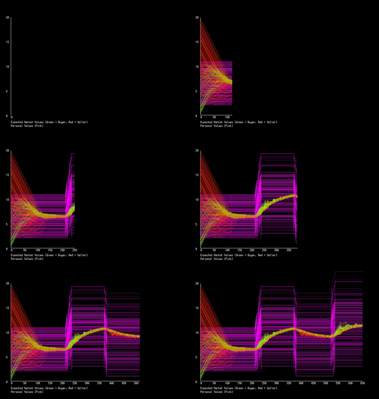
With this very simple decision making process we can run our first simulation. We will have 200 actors in this market, each starting with a random personal value and expected value. Below is the graph of expected values (green and red for buyers and sellers respectively) and personal values (pink). I modify actors personal values at different points in time to see how it effects the market.

We see a quick convergence of expected values to what looks like the average of the personal values. Actually, its converging to the median. Our market applies forces that try and balance the number of buyers and sellers, penalizing those who don’t get matched up. Another perspective we can take is to consider the supply demand curves.

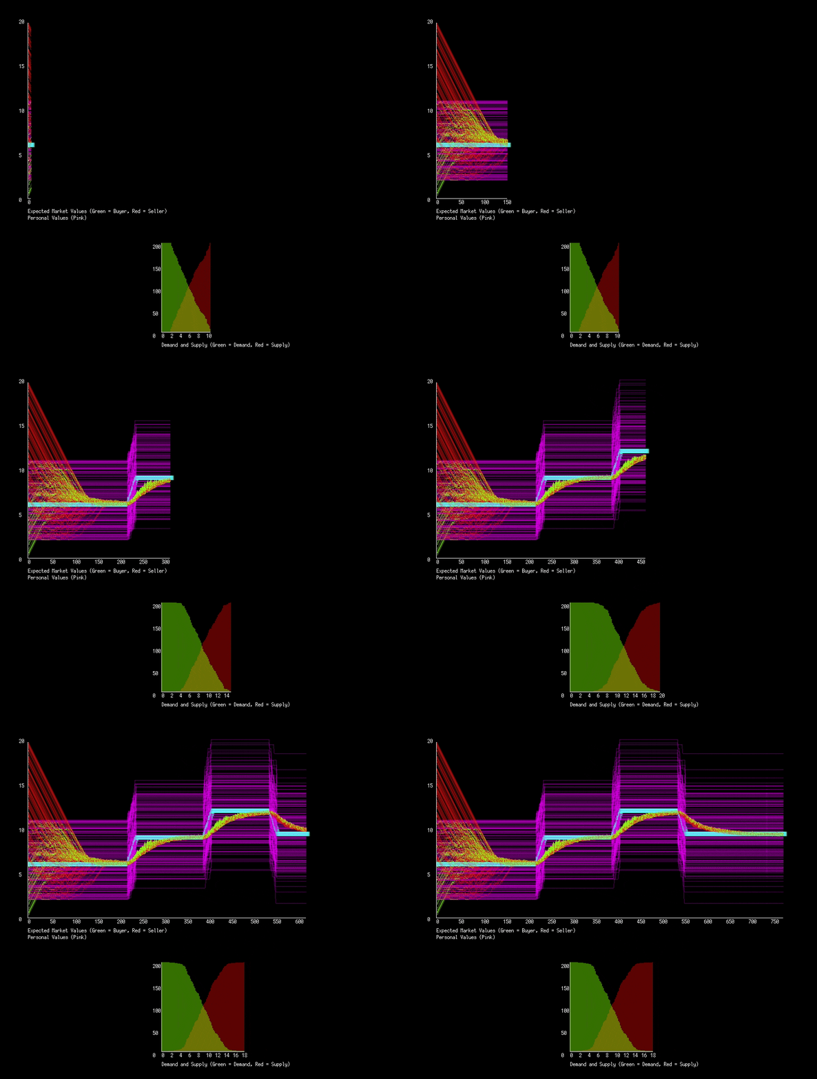
Instead of being given the supply and demand curves, we need to derive them. Given that we know peoples personal values, we can determine for some hypothetical price how many people will be buyers and how many sellers. Graphing for every price the number of buyers will give us a demand curve, and similarly with sellers the supply curve. By finding at what price the two curves are equal, we find the theoretical optimal price. Below is again 200 people interacting every frame, some personal values changed at points in time. We add in the theoretical price to the graph (blue), as well as the supply and demand curves.

The basic principal works well! We haven’t set a global price for a good, or set who should buy or sell, and yet we get a functioning economy that converges to the best possible market price and adapts to changes in actors personal values.

Next

Currently we rely on a round based approach, but economies don’t function in these discrete rounds, people buy and sell at random times. People also don’t transact anything at the moment, they just exchange information, but no goods. Both these issues can be easily addressed, but the second will create a new and interesting problem: Scarcity.