Simulated Economy (8)

Population dynamics

Let us take a detour into the world of ecology, specifically, population dynamics. Ecosystems share that spirit of emergence that we’ve experienced in our simulated economy so far. From small local interactions resulting in large system-wide properties, population dynamics can with just a few simple rules become breathtakingly complex. But not to get ahead of ourselves, let’s start simple.

Rather then simulate the individual agents in populations, like we’ve done in the economy, we shall simulate at the population-wide scale. We justify this by stating that these agents are far more simple then our economic agents, although some interesting properties will be lost (like natural geographic separation for example, or having heterogenous agents). We shall use differential equations to govern the simulation, but fear not, no experience in differential equations is necessary to follow along. As usual, a simple example to begin.

Models

Rabbits are known to proliferate quickly, so if we have $100$ rabbits today, we may have $200$ in 10 days, and then $400$ 10 days after that. In general, if we have $R$ rabbits, then the change in rabbits over time $\frac{dR}{dt}$ is proportional to the number of rabbits we have now multiplied by some constant $a$, which we call the reproduction rate. In code this might look like

R = 100 // initial population
a = 0.005 // fraction of rabbits that reproduce each frame

every frame:
	dR = a * R
	R = R + dR
	plot(R)

All future differential equations can be easily converted into code similar to the above, so we only need to consider the equations from here on out. So for a simple population we have

$\frac{dR}{dt} = aR$

We see here what that population would look like, an exploding number of rabbits in a short period of time (an exponential).

Real rabbits cannot reproduce forever, eventually they run out of room or resources. We create the carrying capacity $K$, this tells us when a population is too large. This can be incorporated into the model as

$\frac{dR}{dt} = aR(1-\frac{R}{K})$

For $R<K$ the change is positive, so the same behavior as before. For $R>K$ the change becomes negative, which means the population will decrease. And so the population always moves towards the carrying capacity.

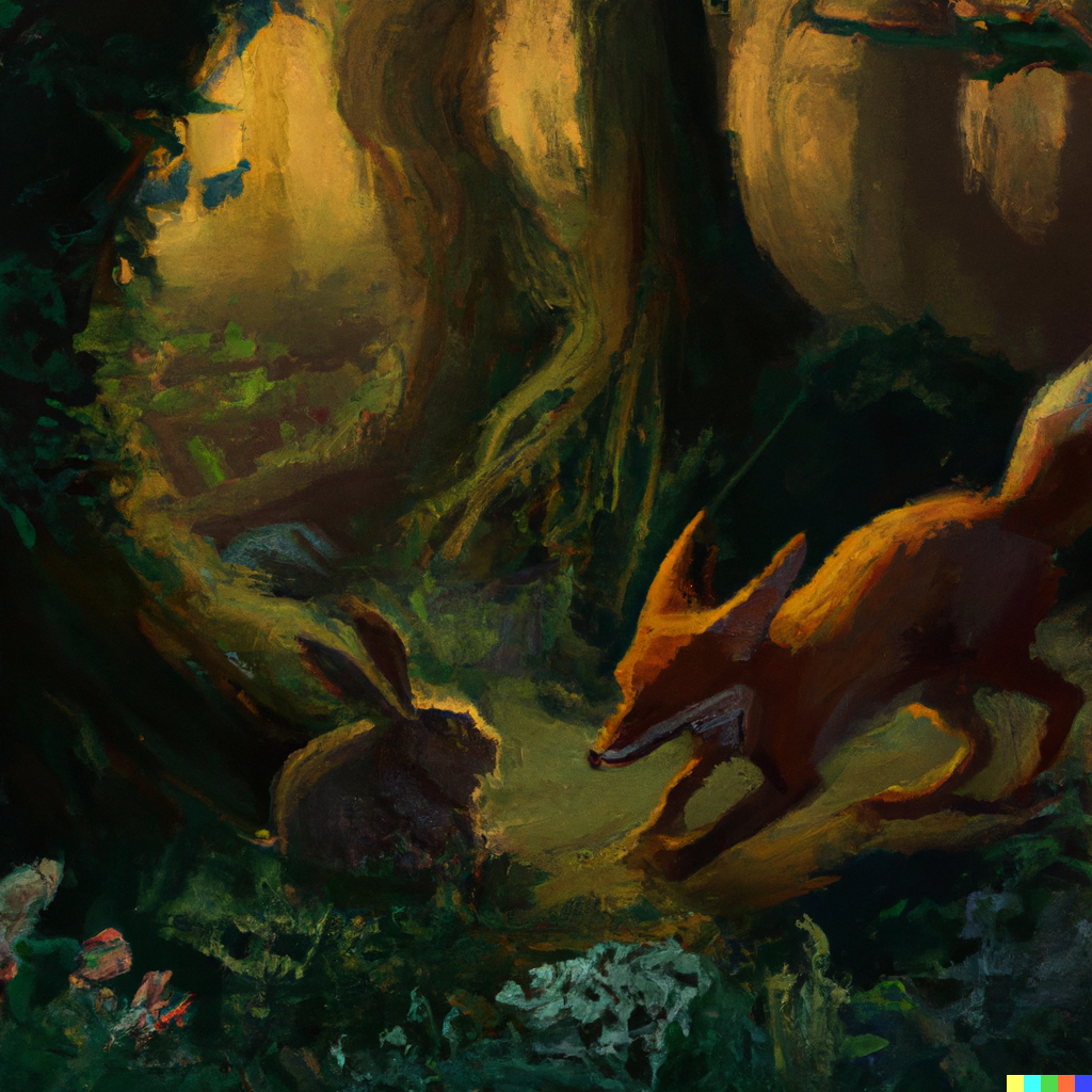
And now we introduce a new population, one that will hunt the rabbits. A population of foxes $F$ will eat rabbits at a rate of $b$, so the rabbit differential equation is now

$\frac{dR}{dt} = aR(1-\frac{R}{K})-bRF$

by subtracting $bRF$, we cause the change of rabbits to be negative when the population of foxes is high (many foxes will eat many rabbits). We include $R$ in $bRF$ since each fox catches a fraction of all rabbits, rather then each fox eating a set number of rabbits.

We also have the fox differential equation. Let $c$ be the death rate of foxes in the absence of any food, and $d$ be the rate of conversion of food (rabbits) into new foxes. No need for carrying capacity since they require rabbits to survive, which have a carrying capacity.

$\frac{dF}{dt} = -cF+dRF$

We can watch the populations interact over time in two ways. One is to plot both populations against time. The other is to plot a point moving over time with coordinates of the population counts, known as the phase space. Let’s view both, with the phase space using coordinates $(R, F)$. Note that different parameters will create different graphs, here we set the carrying capacity to infinity, so it doesn’t effect the rabbit population, what we see is due only to the interaction of the two populations.

We see interesting behavior with the populations, they are both oscillating. This is strange considering we don’t see oscillations defined anywhere in the differential equations. Even more interesting, if we set the carrying capacity of the rabbits to a finite number, then the graph spirals towards a stable point.

And in fact, even if we change the initial conditions, both populations will always spiral towards that same stable point. There are other sets of parameters that will produce limit cycles rather then fixed points, but for this set of parameters, all initial values will converge to the same point.

But how about a third population? If we have grass $G$ which grows into its carrying capacity, rabbits $R$ that eat grass, and foxes $F$ that eat rabbits. All that together we get a 3D system. We will represent the third dimension in the phase space by the size of the point.

$\frac{dF}{dt} = -aFR-bF$

$\frac{dR}{dt} = -cRG-dRF$

$\frac{dG}{dt} = -eG(1-\frac{G}{K})-fGR$

We see another limit point here, so the populations will always converge to these values. We have seen limit points and cycles, but we can also find aperiodic behavior in phase space.

Although I provide no justification, what if the relationship between foxes, rabbits, and grass followed the equations below? We allow values to be negative and simply imagine the graph is shifted, or imagine the numbers represent something other then population size.

$\frac{dF}{dt} = a+F(G-b)$

$\frac{dR}{dt} = G + cR$

$\frac{dG}{dt} = -R - F$

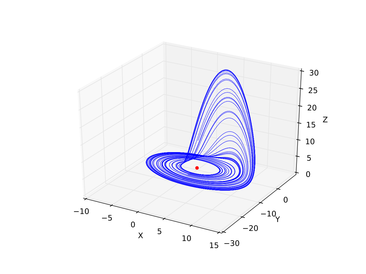
If you plot the path of the point in phase space in three dimensions, you would get the following. Notice how when traveling around the disk that sometimes the Z-axis has a small bump, sometimes a large bump, and sometimes no bump at all. This is exactly what we see when watching the fox population.

This is known as the Rössler attractor, and it’s far from the strangest shape that we can build.

Chaotic attractors

By introducing this third variable we are thrust into the world of chaos theory. Here we find beautiful shapes traced out in phase space, lines that never cross or repeat, but wander along a unique shape, an attractor.

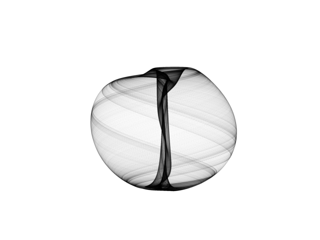
Like with our foxes and rabbits, we can trace a point in phase space according to a set of differential equations. Here we see the continuous 3D chaotic Aizawa attractor.

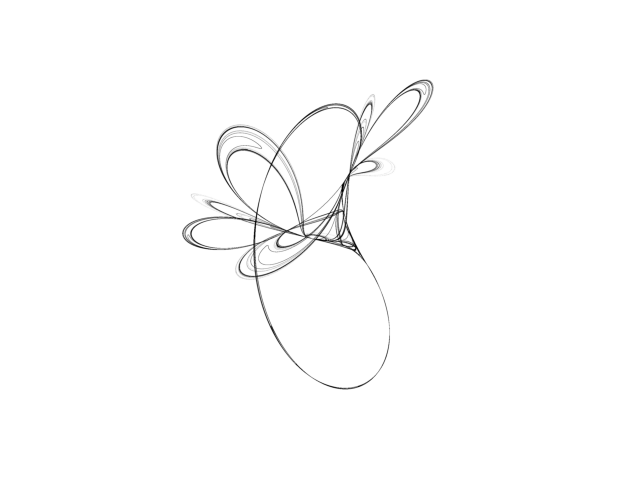
Note that it is necessary to have at least three dimensions for continuous chaotic attractors, but discrete chaotic attractors only need two dimensions. Here we see the Tinkerbell attractor, a discrete 2D chaotic attractor.

Our fox-rabbit-grass simulation is discrete since it’s simulated on a computer run by a clock. There’s nothing stopping us from using a discrete model for our populations (other then trying to fabric a feasible justification for the equations).

We see immense complexity with just three variables, imagine the beauty to be seen in higher dimensions (ah, but we are confined to only shadows of shadows of those possible shapes). But as this relates back to our populations, higher dimensions are trivial to add and view. We would add more populations and watch the population counts change overtime. If we see aperiodic behavior, theres a good chance our populations are a point traveling in phase space along a strange attractor.

Here are some beautiful visualizations of attractors. We can also create attractors that have never been seen before. For a proper introduction to dynamical systems and chaos, check out this free lecture series by Steven Strogatz.

Economy

But we’ve strayed, how does this have anything to do with our simulated economy? Well, in order to assure no one will ever understand what’s going on in our economy, we add chaos.

Starting with our population simulation, we will add one more variable, hunters. Now we have four variables that are all interconnected, humans, foxes, rabbits, and grass. We will use the Rössler attractor to relate the foxes, rabbits, and grass, and humans can kill foxes. Now that we have a sufficiently complex system, let’s connect it to our economy.

We will have the population simulation sit on its own machine that can only be connected to via travleways, which means only merchants can access it (we haven’t added traveling citizens yet). Instead of thread, we have furs, which can only be produced at this hunting grounds. When merchants travel to the hunting grounds, they will randomly kill foxes until they reach their carrying capacity. Their success is in proportion to the number of foxes. When the fox population is high, merchants will quickly reach their carrying capacity and leave, bringing prices down. When the population is low, the merchants will leave slowly, and prices will rise.

We see when the fox population explodes, the price of furs drops, and indirectly the price of beds as well. Every time a fox is killed, it nudges the point in phase space just a bit, completely redirecting the future of the ecosystem (thats what it means to be a chaotic attractor).

We could keep going. There could be chaotic weather systems which effect populations and travel conditions (as it happens, chaos theory was born out of weather models), or the orbits of many planets which effects the day-night cycle and weather conditions, or even the flow of molten iron in the outer core that determine the planets magnetic poles.