I came across an interesting problem in a previous post where boids would get stuck while trying to “vote” on the rotation of a shape. Let’s explore different voting mechanisms in a swarm and see what happens.
Voting Strategies
First let’s look at a simple case: voting on a scalar. Everyone starts with a random number, and then they receive their neighbor’s values every second or so. There are multiple strategies we could choose for what a boid does when receiving a value:
- Highest value: If the incoming value is higher than our current value, then replace our current with that value. This strategy will lead to the group eventually agreeing on the largest value in the swarm.
- Random: Some percent of the time you replace your current value with the incoming value. There is no guarantee the swarm will eventually agree on a value.
- Average: Replace your current value with the average of the incoming value and your current value. This will cause the swarm to eventually all agree on what is essentially the average of all the swarm’s initial values.
For a simplified environment, let’s look at a grid of squares. The squares initialize with random values and will be colored based on their value (grayscale with black as 0 and white as 1). Each square will look at its neighboring squares and use one of the above methods to modify its value. From left to right we see the strategies of Highest, Random, and Average.
We see that only Highest and Average result in all squares reaching agreement, but note that with Average, the values are not exactly the same.
If we consider voting on a vector of scalars we see all the strategies still apply (you could even use different strategies for each dimension).
For labels (like “Apple” and “Orange”) you could only use Random. However, if you create some ordering on the values (so length wouldn’t work since different labels could have the same length, but converting the letters to numbers of a 26-base number system would), then you could use Highest.
For rotations (values on a unit circle) we could use all three strategies, but averaging looks a bit different. Random works for all types of values, Highest can be used by considering the angle as an input, but for Averaging we need a new strategy. The average of 20 degrees and 60 degrees seems simple enough, it should be 40 degrees. But what about the average of 20 degrees and 300 degrees? The correct answer should be 340, not 160. Below we see what averaging on a circle might look like.
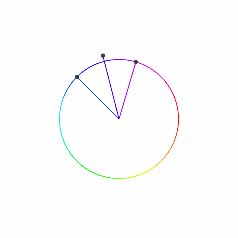
Note that this concept of “averaging” fails when the two values are exactly 180 degrees from each other, which is an edge case we will ignore.
Let’s use this new concept of averaging on the grid of squares, which will now store a rotational value rather than a scalar. Below are the squares running the Average strategy, represented with squares and also with arrows so we can get a more clear idea of what’s going on.
We note some interesting behavior here, specifically that there are these unstable regions where all angles are being voted for, but they don’t always disappear, sometimes they wander. If you look closely you can find three different types: all pointing in or out around a point (sources and sinks), all rotating around a point (rotations), or a saddle point. Keep this in mind for later.
But let’s relate this back to the boids issue that started this all off. Rather than a grid of boids, we were looking at a circle of boids (it was actually an annulus). So let’s run the same simulation as above, but instead of squares on a grid, we use agents on a circle.
On a circle
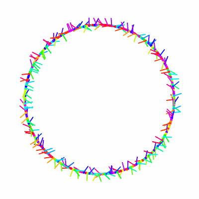
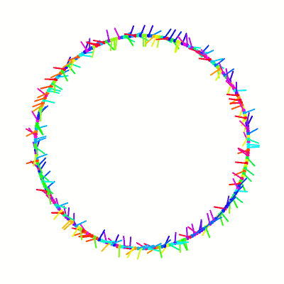
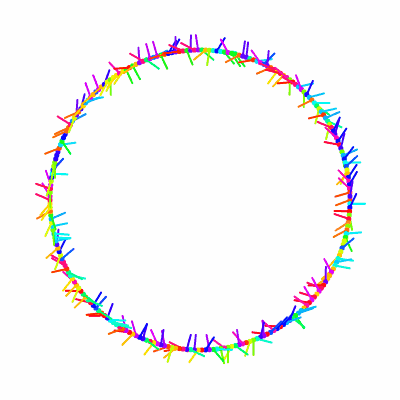
And we see the issue that began this investigation, the agents do not all converge to the same value. Given initially random values, they seem to settle on cycles of the value, the number of cycles different each time. Could we predict what the final result will look like given the initial configuration? Yes!
Let us start at a point on the circle, then add up the change in angle as we travel around the circle (including the angle between the last and first agent). Let’s graph that sum with the x-axis being the angle traveled. We will also draw a vertical line for every 360 degrees on the graph. We know the sum must land on one of these vertical lines (think through with 3 agents to get an intuition of why).
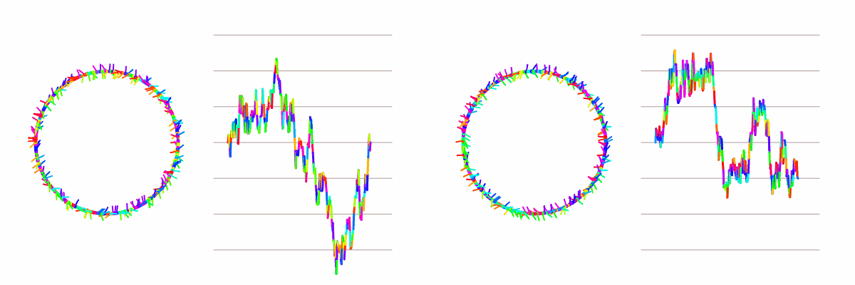
We have on the left a swarm that converges to a single value, and to the right a swarm that converges to one cycle of values. We notice that the swarm that converges to a single value had the sum land on the same vertical line that it started on, while the swarm with a cycle of values had the sum land one vertical line away.
This technique allows us to determine the end result for any initial beliefs and whether they will disagree or not, more than that, how many times they will cycle the disagreement and in what direction.
There is a continuous analog of this problem. If you define a complex function from the agents in their circle (or square, whatever shape they are outlining) to values on the unit circle, then you can consider the function as a curve and find its winding number around 0. Intuitively you can see this below. The agents are in the shape of a diamond outline, and as you travel along that outline you get complex values, which define a curve. The winding number is the mathematical equivalent of counting the number of times a curve travels around a point, and since our curve travels along the unit circle, we can use 0 as our point.
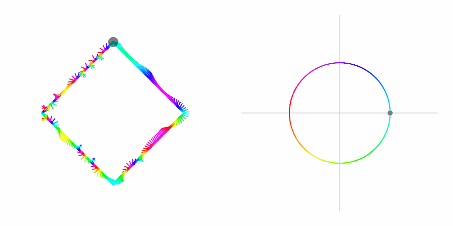
We see the winding number is positive two for this function on the diamond. This tells us the swarm (in the continuous sense) will settle with values cycling twice around the diamond in the clockwise direction.
How might similar issues arise in other shapes and different dimensions? In order to better explore those places it is easier to work in the purely mathematical world.
Continuous function representation
The continuous version of this is where the state of the boids is represented as a continuous function from a surface to the unit circle. For example, the grid of boids represented as 20x20 values on the unit circle would be replaced with a continuous mapping from the unit square to the unit circle.
Already we know this is an approximation, since in the case where the surface was a grid we saw disagreement points (sinks, sources, rotations, saddles), which are not continuous at those points. Physicists study our grid under the name of the XY model and call these points topological defects. We will come back to why the discrete grid gets to have them while the continuous world does not. For now let us ignore the discrepancy and play in this new space.
What we need to do is imagine all the possible continuous functions from the surface to the unit circle, then imagine the limit as those functions change according to the averaging strategy, and then ask whether any limits exist which are not just the constant function. This tells us if it’s possible for the boids’ beliefs to be permanently twisted when placed in the given shape.
Take the diamond outline we’ve seen above. There are many functions which in their limits are the constant function, anything with a winding value of 0. But then there are functions whose limit is not constant, namely those with non-zero winding values. Mathematicians have a name for the thing separating these two groups: homotopy. Two functions are homotopic if one can be continuously deformed into the other, and the resulting families of mutually-deformable functions are called homotopy classes. Notice that averaging is itself a continuous deformation, so a swarm can never leave the homotopy class it started in. On the diamond, the homotopy classes are exactly the winding numbers, one class for each integer, and only class 0 contains the constant function. A swarm that starts with winding number 2 is trapped with winding number 2 forever.
On the square (continuous version of the grid), I can’t imagine any function whose limit is not the constant function. Similarly for the sphere. See if you can imagine a continuous assignment of unit circle values over the sphere that allows for some closed curve on the sphere to produce a non-zero winding number.
This turns out not to be possible: every state on the sphere has a winding value of 0 along every closed curve. We can show this using two facts: the winding value on any closed curve over the surface stays constant as the swarm averages, and the winding value does not change as you smoothly deform the curve. Both of these facts follow from one observation: The winding number is an integer, and an integer cannot change continuously. Deforming the curve is a continuous process. Averaging the function is a continuous process. Neither can move an integer, so neither can change the winding number. In the language above, the winding number is a homotopy invariant.
Now the argument for the sphere goes through. If the sphere admitted a non-constant limit, there would exist some closed curve with a non-zero winding value. But every closed curve on the sphere can be smoothly deformed into an arbitrarily small circle, and a small enough circle on a continuous function must have a winding value of 0. So every curve had a winding value of 0 all along, and so the limit of any initial state on the sphere will converge to the constant function. The same argument works on the square.
There is a general theorem that encompasses these examples. The homotopy classes of continuous functions from a space $X$ to the unit circle correspond exactly to the elements of a group called the first cohomology group $H^1(X; \mathbb{Z})$. We don’t need the machinery here, but the takeaway is: the group is computable from the shape alone, and it roughly counts the independent ways to loop around holes in the shape. The circle (or diamond, any loop) has one hole, so the group is $\mathbb{Z}$, and disagreement comes in integer amounts. The square and sphere have no holes, so the group is trivial, and agreement is the only outcome. A torus has two independent loops, so its configurations are classified by a pair of integers, one winding count around each direction. We can now predict the fate of a swarm on any surface without running a single simulation. The shape alone tells us the possible homotopy classes, and therefore whether the swarm can ever get permanently stuck.
But if we did need to define a smoothing function on the state (a continuous function from a surface to the unit circle) to create the continuous version of the averaging strategy, what might it look like? I like to imagine the unit circle values as vectors, where we can apply the heat equation to each component every timestep, then project the results back onto the unit circle. This is an approximation of the real thing, a process called the harmonic map heat flow, which is the heat equation plus a correction term that keeps the values on the circle at every instant rather than fixing them afterward. Eells and Sampson introduced it in 1964 and proved that when the target space is not positively curved (which includes our unit circle, so the theorem applies to us), the flow runs forever and converges to the minimum-energy function within the starting homotopy class. On a loop with winding number $q$, that minimizer is the uniform twist, values rotating $q$ times at a constant rate. In class 0, it is the constant function. This is exactly what our simulations found.
Which leaves the loose end from the start of this section, the defect points we saw on the grid. The continuous theory forbids them, but a grid is not continuous. Neighboring squares are separate agents taking finite jumps, so there is no continuity to violate, and the sinks, sources, rotations, and saddles can exist. The topology still constrains them though. Each defect carries an index, the winding number of a small loop drawn around it, and the sum of the indices in any region must equal the winding number around the region’s boundary. A region whose boundary reads 0 can hold defects, but only in canceling pairs. That is why the defects wander and annihilate with their opposites rather than vanishing on their own.
The shape of the swarm determines whether its members can ever agree: if the surface they form has a hole to wind around, some initial beliefs can stay twisted forever, and if it does not, averaging will always bring them to a single value.